Introduction
Natural language processing (NLP) is a branch of artificial intelligence that helps computers comprehend and interact with human language.
In this article, I’ll explain 9 fundamental techniques utilized across NLP models and applications.
And to showcase the practical implementation, I leverage 3 widely used NLP libraries: Natural Language Toolkit (NLTK), Gensim and spaCy. These libraries are designed to streamline text preprocessing, effectively transforming free-form text into structured features that can easily be fed into Machine Learning (ML) or Deep Learning (DL) pipelines.
9 techniques I am going to cover include:
- Tokenization
- Part-of-Speech (POS) Tagging
- Stemming and Lemmatization
- Stop Words
- Bag of Words (BoW)
- TF-IDF
- N-grams
- Word Embeddings
- Named Entity Recognition
So, grab your coffee and let’s get started!
1. Tokenization
The first step in analyzing any text with NLP is to break it down into smaller chunks called tokens. Tokens can be sentences, individual words, characters, or sub-words. Common approaches include splitting text into words, characters, or n-grams. For many languages, words work well as tokens. But for languages like Chinese, individual characters are more meaningful tokens.
Both NLTK and spaCy are powerful tools for tokenization and various other NLP tasks — let’s try them both!
import nltk
from nltk.tokenize import word_tokenize
import spacy

# Load the English language model in spaCy
nlp = spacy.load("en_core_web_sm")

text = "Tokenization is a key process in NLP. Let's see how it's #working."

# Tokenize using nltk
nltk_tokens = word_tokenize(text)

# Tokenize using spaCy
spacy_sent = nlp(text)
spacy_tokens = [token.text for token in spacy_sent]

print("NLTK Tokens:", nltk_tokens)
print("spaCy Tokens:", spacy_tokens)
NLTK Tokens: ['Tokenization', 'is', 'a', 'key', 'process', 'in', 'NLP',
'.', 'Let', "'s", 'see', 'how', 'it', "'s", '#', 'working', '.']
spaCy Tokens: ['Tokenization', 'is', 'a', 'key', 'process', 'in', 'NLP',
'.', 'Let', "'s", 'see', 'how', 'it', "'s", '#', 'working', '.']Observation
- You may notice that both NLTK and spaCy consider punctuation, which is ‘#’ in the example above, as a token. To eliminate unnecessary symbols and make the text cleaner and simpler, we can perform punctuation removal before tokenization.
import string

exclude = set(string.punctuation)
print(f"Punctuation list: {exclude}")

text_no_punc = ''.join(ch for ch in text if ch not in exclude)
print(f"Original text: {text}")
print (f"Text w. no punctuations: {text_no_punc}")

# Tokenize into words
words = word_tokenize(text_no_punc)
print("Tokens w. no punctuations:", words)
Punctuation list: {'^', '.', '}', '"', '-', '&', '$', '@', '?', ']', '>',
'`', '[', '#', '+', ')', ';', '%', '!', '*', '_', '<', '~', '(', ',', ':',
'=', '|', '\\', "'", '{', '/'}
Original text: Tokenization is a key process in NLP. Let's see how
it's #working.
Text w. no punctuations: Tokenization is a key process in NLP Lets see how
its working
Tokens w. no punctuations: ['Tokenization', 'is', 'a', 'key', 'process',
'in', 'NLP', 'Lets', 'see', 'how', 'its', 'working']Observation
- After removing punctuations from the sentence “Let’s see how it’s #working.”, it becomes “Lets see how its working”, and then tokenization generates [‘Lets’, ‘see’, ‘how’, ‘its’, ‘working’]
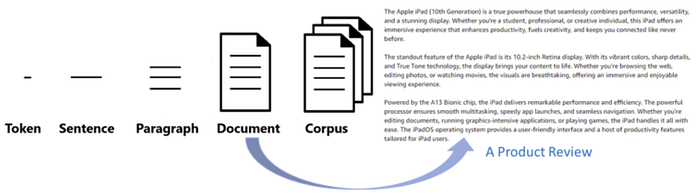
Terminologies
Corpus > Document > Paragraph > Sentence > Token
- Corpus is the collection of text documents.
- Document: A unit of text, such as a tweet, news article or product review.
- Paragraph: A section within a document.
- Sentence: A sequence of words conveying a complete thought.
- Token: The smallest unit after tokenization, representing individual words, characters, or n-grams.
2. Part-of-Speech (POS) Tagging
One of the core tasks in NLP is Parts of Speech (PoS) tagging, which is giving each word in a text a grammatical category, such as nouns, verbs, adjectives, and adverbs. This technique helps machines to study and comprehend human language more accurately, it is a link between machine and language.
PoS tagging is essential in many NLP applications, including machine translation, named entity recognition, sentiment analysis, and information retrieval.
import nltk
from nltk.tokenize import word_tokenize

# Sample sentence
sentence = "John likes to watch action movies. I like playing soccer"

# Tokenize the sentence into words
tokens = word_tokenize(sentence)

# Perform POS tagging
pos_tags = nltk.pos_tag(tokens)

# Display POS tagged tokens
print(pos_tags)
[('John', 'NNP'), ('likes', 'VBZ'), ('to', 'TO'), ('watch', 'VB'),
('action', 'NN'), ('movies', 'NNS'), ('.', '.'), ('I', 'PRP'),
('like', 'IN'), ('playing', 'VBG'), ('soccer', 'NN')]Each word is paired with its corresponding POS tag. For instance:
- ‘John’ is tagged as ‘NNP’ (proper noun, singular).
- ‘likes’ is tagged as ‘VBZ’ (verb, third person singular present).
- ‘to’ is tagged as ‘TO’ (to).
- ‘watch’ is tagged as ‘VB’ (verb, base form).
- ‘movies’ is tagged as ‘NNS’ (noun, plural).
- ‘action’ is tagged as ‘NN’ (noun, common, singular or mass)
- ‘.’ is tagged as ‘.’ (punctuation).
We can use function nltk.help.upenn_tagset() to get all the tags in nltk library.
3. Stemming and Lemmatization
Lemmatization and Stemming are text normalization techniques. In any languages, there are many words derived from some root forms and we will try to get the root forms using Stemming and Lemmatization. The purpose of these 2 techniques is quite similar, so what is the difference?
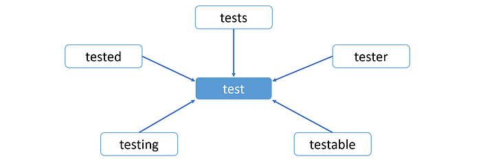
Stemming is a technique that reduces a word to its root form using rules and lists of known suffixes. The root form may or may not be a legitimate word in the language. For instance, the stem of these five words ‘testing’, ‘tested’, ‘tests’, ‘testable’, ‘tester’, is ‘test’.
In stemming, a part of the word is just chopped off at the tail end to arrive at the stem of the word. There are different algorithms, as you can see later, used to find out how many characters have to be chopped off, but the algorithms don’t actually know the meaning of the word.
The code below demonstrates how to perform 3 stemming algorithms using NLTK and conducts a comparative analysis of the outcomes.
The first stemming algorithm is Porter Stemming which was created by Martin Porter in 1980 and widely used since then.
Snowball Stemming was also created by Martin Porter. The method utilized in this instance is more precise and is referred to as “English Stemmer” or “Porter2 Stemmer.” It is faster and more logical than the original Porter Stemmer. As of now, Snowball Stemming is supporting 16 languages, such as Arabic, German, French, Russian … so we have to specify the language that we are stemming while initializing the stemmer object.
The Lancaster Stemming algorithm is known to be more aggressive than other stemming algorithms, such as the Porter and Snowball algorithms. We can see the results in the column Lancaster below.
from nltk.stem import PorterStemmer
from nltk.tokenize import word_tokenize
from nltk.stem import SnowballStemmer
from nltk.stem import LancasterStemmer

# Sample text
text = "Lemmatization important language techniques. " \
       "Caring testable eaten was beautifully better driver"

# Tokenizing the text
tokens = word_tokenize(text)

# Stemming in 3 ways
porter = PorterStemmer()
snowball = SnowballStemmer(language='english')
lancaster = LancasterStemmer()

print("{0:16}{1:16}{2:18}{3:18}".
      format("Word","Porter","Snowball","Lancaster"))
for w in tokens:
    print("{0:16}{1:16}{2:18}{3:18}".
          format(w,porter.stem(w),snowball.stem(w),lancaster.stem(w)))
Word Porter Snowball Lancaster
Lemmatization lemmat lemmat lem
important import import import
language languag languag langu
techniques techniqu techniqu techn
. . . .
Caring care care car
testable testabl testabl test
eaten eaten eaten eat
was wa was was
beautifully beauti beauti beauty
better better better bet
driver driver driver driv Observations
- languag, langu, techniqu, wa, beauti, driv are not recognized words.
- import (stem of important) might be confused with the correct import. “important step in importing process” after being stemmed becomes “import step in import process”.
- Stemming algorithms only reduce the suffixes, not prefixes.
Stemming is not a perfect process, however, stemming is still a useful tool for reducing the dimensionality of text data and transforming words into a common format for processing.
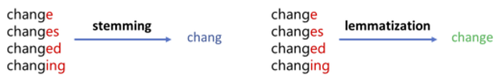
Lemmatization is a text pre-processing technique that considers the context and uses a comprehensive full-form dictionary to understand the meaning of the word to return the base or dictionary form of a word. So, a lemmatization algorithm would know that the word 'better' is derived from the word ‘good’, and hence, the lemme of ‘better’ is 'good'. The lemma of ‘am’, ‘are’, ‘is’, ‘were’, ‘was’, ‘been’ is 'be'. But there is no way in stemming that can reduce ‘were’ to ‘be’, stemming just chop the tail of the word.
The root word is called a stem in the stemming process, and it’s called a lemma in the lemmatization process.
As opposed to stemming, lemmatization relies on accurately determining the Part-of-speech (PoS, explained in the next section) and the meaning of a word based on its context. This means it takes into consideration the position of the inflected word within a sentence, as well as within the larger context surrounding that sentence. I have created a weird text below and let’s see how lemmatization analyzes it.
import spacy

# Load the English language model in spaCy
nlp = spacy.load('en_core_web_sm')

# Sample text
text = "The caring driver, who had the best intentions, drove cautiously,"\
       "but the results were changed. Caring about him."

# Process the text using spaCy
doc = nlp(text)

# Lemmatization using spaCy
lemmatized_words = [token.lemma_ for token in doc]

print(f"Lemmatized Words:\n{lemmatized_words}")
Lemmatized Words:
['the', 'caring', 'driver', ',', 'who', 'have', 'the', 'good', 'intention',
',', 'drive', 'cautiously', ',', 'but', 'the', 'result', 'be', 'change',
'.', 'care', 'about', 'he', '.']Observations
- ‘Caring’ has 2 different lemmas as one of them is adjective and the other is V-ing.
- Stem of ‘best’ is itself, but lemma of ‘best’ is ‘good’.
- Lemma of ‘driver’ (noun) is itself. Lemma of ‘drove’ (verb, past tense) is ‘drive’.
Differences between Stemming and Lemmatization
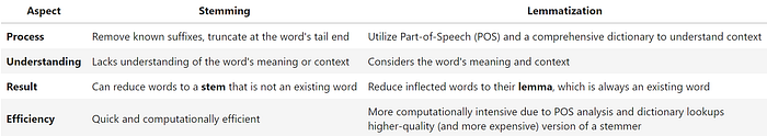
We can consider a lemmatizer as a higher-quality (and more expensive) version of a stemmer. However, in most machine learning problems, computational resources are rarely a cause for concern.
4. Stop Words
Commonly used words (e.g., “the,” “and,” “is”, “couldn’t”, “over”, etc.) that are often filtered out in NLP tasks due to their high frequency and low informational value.
There are many stop word lists available and I used stop words from nltk.corpus in my example to prevent all words in the stop word list from being analyzed.
import nltk
from nltk.corpus import stopwords
from nltk.tokenize import word_tokenize

text = "How did you collect those books in Eugene?"

# Tokenizing the text
tokens = word_tokenize(text)

# Getting English stopwords from NLTK
stop_words = set(stopwords.words('english'))

# Removing stop words from the tokens
filtered_tokens = [w for w in tokens if w.lower() not in stop_words]

print(f"Original Tokens: {tokens}")
print(f"After Removing Stop Words: {filtered_tokens}")
Original Tokens: ['How', 'did', 'you', 'collect', 'those', 'books',
'in', 'Eugene', '?']
Tokens after Removing Stop Words: ['collect', 'books', 'Eugene', '?']On the other hand, some stop words play an important role in the sentence, helping the model better understand the context. For example, what remains after removing stop words from the text above are just ‘collected’, ‘books’, ‘Eugene’, ‘?’. If we know that it is a ‘How’ or ‘Why’ or ‘Where’ question (e.g., Why did you collect those books for Eugene?), we can generate a better results for users.
Word Vectorization and Word Embedding
Machine learning with natural language encounters with a major challenge — its algorithms typically handle well-defined, fixed-length inputs and outputs of numbers, while natural language is, well, text. Therefore, we must transform all the words into vectors of numbers, the process is called word vectorization.
Word Vectorization is the general term that includes embedding and other simpler approaches.
- Bag of Words (BoW) is a simple approach which convert words or text documents into sparse and high-dimensional vector space (e.g., 100,000 dimensions), where each dimension corresponds to a unique word. There are 2 scoring methods in BoW: Count Vector and TF-IDF.
- Word Embedding transform words into dense, low-dimensional, continuous-valued vectors in a continuous vector space. Similar words or words with related meanings are placed closer together in the embedding space. Some popular Word embedding techniques are Word2Vec, GloVe, BERT and FastText. Among them, Word2Vec and FastText use neural networks to learn the vectorization.
I will explain about Bag of Words, TF-IDF and Word Embedding in the next sections.
5. Bag of Words (BoW) with Count Vector
A popular and straightforward method of converting text data into vectors (aka. feature extraction) is called the bag-of-words model of text.
A bag-of-words is a representation of text that captures the occurrence of words within a document. It involves two key components:
- A vocabulary of known words.
- A measure of the presence of these known words.
It is called a “bag” of words, because any information regarding the order or structure of words in the document is discarded. The model focuses only on whether known words occur in the document, not where in the document.
from sklearn.feature_extraction.text import CountVectorizer

# Sample text data
text_data = [
    "It was the best of times",
    "it was the worst of times",
    "it was the age of wisdom",
    "it was the age of foolishness was"  # added an extra "was"
]

# Create an instance of CountVectorizer
vectorizer = CountVectorizer()

# Transform the text data into a sparse matrix of token counts
bow_matrix = vectorizer.fit_transform(text_data)

# Get the feature names (vocabulary)
feature_names = vectorizer.get_feature_names_out()

# Convert the sparse matrix to an array for readability
bow_array = bow_matrix.toarray()

# Display the vocabulary (unique words)
print("Vocabulary:\n", feature_names)

# Display the BoW matrix
print("BoW Document Term Matrix:\n", bow_array)
Vocabulary:
['age' 'best' 'foolishness' 'it' 'of' 'the' 'times' 'was' 'wisdom' 'worst']
BoW Document Term Matrix:
[[0 1 0 1 1 1 1 1 0 0]
[0 0 0 1 1 1 1 1 0 1]
[1 0 0 1 1 1 0 1 1 0]
[1 0 1 1 1 1 0 2 0 0]]That is a vocabulary of 10 words from a corpus containing 24 words. The next step is to score the words in each document. The goal is to transform each document of free text into a vector that we can use as input for a machine learning model. Given the 10-word vocabulary, we can use a fixed-length document representation of 10, with one position in the vector to score each word.
In the given example, Count Vector method is used to score the words. CountVectorizer creates a document term matrix in which the individual cells denote the frequency of that word in a particular document, which is also known as term frequency, and the columns are dedicated to each word in the corpus.
Observations
- The vectors represented for the first 2 documents (or sentences) are closer to each other, this will help in text classification.
- The last document has 2 ‘was’ so the last row of the matrix has number 2 at ‘was’ column.
You can imagine that for a very large corpus, such as thousands of books, the vocabulary size would increase and cause vector length of thousands or millions of positions. Moreover, each document may contain only a few of the known words in the vocabulary, leading to a vector with lots of zero scores, called a sparse vector.
With the above vocabulary, the vector for the word ‘best’ would be [0,1,0,0,0,0,0,0,0,0] and ‘worst’ would be [0,0,0,0,0,0,0,0,0,1] (One-hot encoding) — there is clearly no relationship between the 2 words.
Sparse vectors require more memory and computational resources when modeling and the vast number of positions or dimensions can make the modeling process very challenging for traditional algorithms. As such, there is pressure to decrease the size of the vocabulary when using a bag-of-words model. There are simple text cleaning techniques that can be used as a first step, such as:
- Ignoring case
- Ignoring punctuation
- Ignoring frequent words that don’t contain much information, called stop words, like “a,” “of,” etc.
- Fixing misspelled words.
- Reducing words to their stem (e.g. “play” from “playing”) using stemming algorithms.
6. TF-IDF
BOW with Count Vector method is simple and works well, but the problem with that is that it treats all words equally. Highly frequent words dominate in the document (e.g. larger score), but may not contain as much “informational content” to the model as rarer but perhaps domain specific words.
Another scoring method in BoW is to rescale the frequency of words by how often they appear in all documents, so that the scores for frequent words like “the” that are also frequent across all documents are penalized.
This approach is called Term Frequency — Inverse Document Frequency, or TF-IDF for short, where:
- Term Frequency: is a scoring of the frequency of the word in the current document.
- Inverse Document Frequency: is a scoring of how rare the word is across documents. The intuition behind Inverse Document Frequency is that the more common a word is across all documents, the lesser its importance is for the current document. The more common a word is, the closer it is to 0.
Multiplying these two numbers results in the TF-IDF score of a word in a document. The higher the score, the more relevant that word is in that particular document.
“Thus the IDF of a rare term is high, whereas the IDF of a frequent term is likely to be low.” — Christopher D. Manning
Converts the documents into TF-IDF vectors and then retrieves the TF-IDF scores for each word in each document.
from sklearn.feature_extraction.text import TfidfVectorizer

# Sample documents
documents = [
    'This is the first document.',
    'This document is the second document.',
    'And this is the third third third one.',  # added 2 extra "third"
    'Is this the first document?',
]

vectorizer = TfidfVectorizer()

# Fit and transform the documents to TF-IDF vectors
tfidf_vectors = vectorizer.fit_transform(documents)

# Get the vocabulary (unique words)
words = vectorizer.get_feature_names_out()

# Create a dictionary to store TF-IDF scores for each word in each document
tfidf_scores = {}
for i, doc in enumerate(documents):
    feature_index = tfidf_vectors[i, :].nonzero()[1]
    tfidf_doc = zip([words[idx] for idx in feature_index],
                    [tfidf_vectors[i, x] for x in feature_index])
    tfidf_scores[i] = {word: score for word, score in tfidf_doc}

# Print TF-IDF scores for each word in each document
for doc_id, scores in tfidf_scores.items():
    print(f"Document {doc_id + 1}:")
    for word, score in scores.items():
        print(f"\t{word}: {score:.4f}")
TF-IDF assigns a high value for a word that is frequent within a single document (high TF), and an even larger value if that word is rare across the entire document set (high IDF).
The first 4 columns D1-4 of the table below are number of word in each document from BoW model. The last 4 columns are TF-IDF scores for words in each document. “-” is the 0 score.
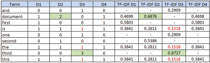
Observations
- 2 words having the highest TF-IDF scores are ‘document’ (showing in three documents with 2 times in D2) and ‘third’ (showing in only one document with 3 times in D3)
- 3 words having the lowest TF-IDF scores are ‘is’, ‘the’ and ‘this’, they are showing in all 4 documents and 1 time each.
TF-IDF is commonly used in document classification, information retrieval, and tasks where word importance based on frequency is crucial.
7. N-grams
A more sophisticated approach of Bag of Words is to create a vocabulary of grouped words. This both changes the scope of the vocabulary and allows the bag-of-words to capture a little bit more meaning from the document.
In this approach, each word or token is called a “gram”. Creating a vocabulary of two-word pairs is, in turn, called a bigram model.
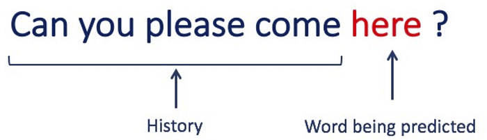
- A 1-gram (or unigram) is a one-word sequence, the unigrams would simply be ‘Can’, ‘you’, ‘please’, ‘come’, ‘here’.
- A 2-gram (or bigram) is a two-word sequence of words, like ‘Can you’, ‘you please’, ‘please come’, ‘come here’.
- A 3-gram (or trigram) is a three-word sequence of words like ‘Can you please’, ‘please come here’, …
N-grams helps us to predict the probability of seeing a word given a history of previous words.
“You shall know the nature of a word by the company it keeps.” — John Rupert Firth
This code snippet uses the NLTK library in Python to generate word-level N-grams from a given text. It tokenizes the text into words using word_tokenize() from NLTK, then utilizes nltk.util.ngrams() to generate N-grams of the specified size (N). Adjust the value of N to create different N-grams (e.g., bigrams, trigrams, etc.).
from nltk.util import ngrams
from nltk.tokenize import word_tokenize
text = "I love reading books about human history."
tokens = word_tokenize(text)# Define the N for N-grams (e.g., bigrams, trigrams, etc.)
N = 2# Generate N-grams
word_ngrams = list(ngrams(tokens, N))print(f"{N}-grams:")
for gram in word_ngrams:
print(gram)
2-grams:
('I', 'love')
('love', 'reading')
('reading', 'books')
('books', 'about')
('about', 'human')
('human', 'history')
('history', '.')
Why do we need n-grams?
Bag of n-grams is a natural extension of bag of words. Bag of n-grams can be more informative than bag of words because they capture words that occur often together and capture more context around each word (i.e. “love reading books” is more informative than just “reading”). However, this comes at a cost as bag of n-grams can produce a much larger and sparser feature set than bag of words.
8. Word Embeddings
Word embeddings are a type of word representation that allows words with similar meaning to have a similar representation. Word embeddings are in fact a class of techniques where individual words are represented as real-valued vectors in a predefined vector space. Each word is represented by a real-valued vector, often tens or hundreds of dimensions. This is contrasted to the thousands or millions of dimensions required for sparse word representations, such as a one-hot encoding. The feature vector represents different aspects of the word: each word is associated with a point in a vector space. The number of features (e.g., 100 or 300) is much smaller than the size of the vocabulary.
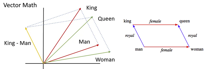
The distributed representation is learned based on the usage of words. This allows words that are used in similar ways to result in having similar representations, naturally capturing their meaning. For example, the male/female relationship is automatically learned, and with the induced vector representations, “King — Man + Woman” results in a vector very close to “Queen”.
Mapping words or phrases from a vocabulary to numerical vectors in a continuous vector space, capturing semantic relationships between words.
Word embedding methods learn a real-valued vector representation for a predefined fixed sized vocabulary from a corpus of text. The learning process is either joint with the neural network model on some task, such as document classification, or is an unsupervised process, using document statistics.
Word2Vec is a statistical method to learn a standalone word embedding from a text corpus. It was developed by Mikolov at Google in 2013. The presentation of “King — Man + Woman = Queen” has been firstly introduced by Word2Vec.
I use Word2Vec to perform word embedding on the Brown corpus, a widely recognized corpus which has one million words. The corpus is made up of about 500 samples from a variety of sources, each almost exactly 2000 words in length. How to use corpus and other corpuses in nltk package can be found here https://www.nltk.org/howto/corpus.html
from gensim.models import Word2Vec
from nltk.corpus import brown

sents = brown.sents()

model = Word2Vec(sentences=sents, vector_size=100, window=3, min_count=1)
print(model)

# Getting the word vectors
word_vectors = model.wv
Word2Vec<vocab=56057, vector_size=100, alpha=0.025>Within that corpus, there are 56,057 unique words. I setup Word2Vec so that each word is represented by a 100-dimensional vector through the embedding process.
Let’s see if the formula “King — Man + Woman = Queen” is correct after the embedding process on the Brown corpus.
output = word_vectors.most_similar(positive=['woman', 'king'],
                                   negative=['man'], topn=3)
print(f"king - man + woman = {output}")

print(f"similarity('king', 'queen'):{model.wv.similarity('king','queen')}")
print(f"similarity('best', 'worst'):{model.wv.similarity('best','worst')}")
print(f"similarity('best', 'was'): {model.wv.similarity('best', 'was')}")

# Finding similar words
similar_words = word_vectors.most_similar("Paris", topn=3)

print(f"Words similar to '{word}': {similar_words}")
king - man + woman = [('inventor', 0.927), ('Academy', 0.921),
('throats', 0.92)]
similarity('king', 'queen'): 0.932
similarity('best', 'worst'): 0.789
similarity('best', 'was'): 0.402
Words similar to 'Paris': [('Rome', 0.981), ('London', 0.981),
('Boston', 0.976)]Observations
- ‘King ‘— ‘Man’ + ‘Woman’ is not close enough to ‘Queen’, we might need to use a much larger corpus so extract better relationship between words. However, ‘king’ and ‘queen’ themselves have a really high similarity.
- In Bag of Words, there is no relationship between ‘best’ and ‘worst’. However, with word embedding, this pair has a much higher similarity than a random pair.
- It makes sense that ‘Paris’ is similar to ‘Rome’, ‘London’ and ‘Boston’. Though, ‘Washington DC’ is obviously a better choice here than ‘Boston’.
9. Named Entity Recognition (NER)
NER extracts and categories entities in a text into predefined categories. The category can be Organization, Event, Person, Location, Date, etc. If your task is to find out ‘where’, ‘what’, ‘who’, ‘when’ from a text, NER is the solution you want to try. It will help users or models focus on essential information.
There are several open-source libraries for NER, in this example, I use a small model (‘_sm’) from spaCy. You can try with ‘_md’ and ‘_lg’ to see if you can have a better result.
import spacy

# Load the English language model in spaCy
NER = spacy.load("en_core_web_sm")

# Sample text for named entity recognition
text = "Apple is a technology company based in Cupertino, California, " \
       "founded by Steve Jobs 48 years ago."
text2 = "Daniel McDonald's son went to McDonald's and ordered a Happy Meal"

# Process the text using spaCy
doc = NER(text)

# Extract named entities and their labels
named_entities = [(entity.text, entity.label_) for entity in doc.ents]

# Print named entities and their labels
for entity, label in named_entities:
    print(f"Entity: {entity}, Label: {label} ({spacy.explain(label)})")
Entity: Apple, Label: ORG (Companies, agencies, institutions, etc.)
Entity: Cupertino, Label: GPE (Countries, cities, states)
Entity: California, Label: GPE (Countries, cities, states)
Entity: Steve Jobs, Label: PERSON (People, including fictional)
Entity: 48 years ago, Label: DATE (Absolute or relative dates or periods)text2 is a tricky sample with 2 different “McDonald’s” but spaCy is able to detect that, let’s see the output below.
Entity: Daniel McDonald's, Label: PERSON (People, including fictional)
Entity: McDonald's, Label: ORG (Companies, agencies, institutions, etc.)
Entity: a Happy Meal, Label: WORK_OF_ART (Titles of books, songs, etc.)
In the upcoming article, I will apply these NLP techniques to preprocess text before categorizing news. See you there!